NASA SPICE Kernels
SPICE kernels are not trivial in their ease of use in their raw format and, thankfully, NASA provides WebGeocalc, a web-based GUI to assist in processing the desired data:
![]()
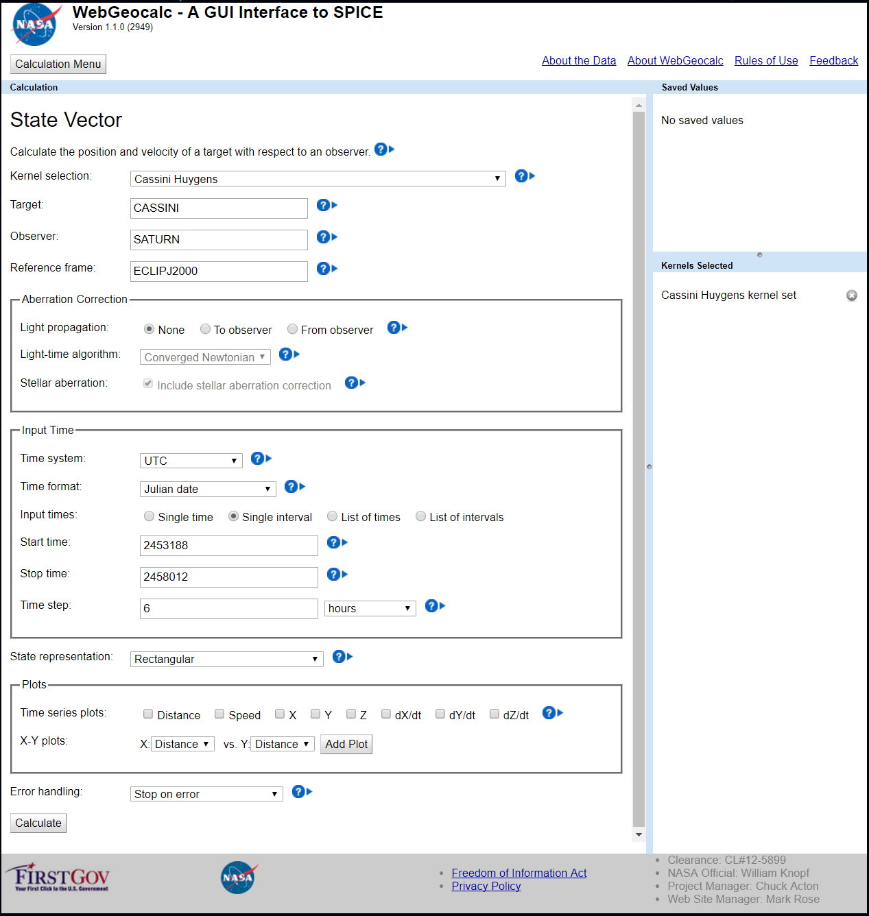
After navigating to the WebGeocalc GUI:
- Choose the kernel set to be "Cassini Huygens." Hovering the mouse over the Cassini Huygens kernel, text is displayed describing an archived kernel including a date range from 10/15/97 until 12/31/2016 (at the time this was published).
- The target should be "CASSINI" (not to be confused with "CASSINI PROBE" which is the Huygens lander), as this is what we are interested in tracking through our reference frame.
- The observer in our case will be "SATURN" (not to be confused with "SATURN BARYCENTER" which includes the center of mass of the Saturnian system) as the reference frame in WWT is centered on Saturn's individual center of mass.
- The reference frame should be specified as "ECLIPJ2000," which is the standard for most cases.
- Aberration Correction can be ignored for our purposes.
- The time system default of "UTC" should be paired with a time format of "Julian Date."
- We want to visualize Cassini's orbital trajectories relative to Saturn beginning with its initial orbital insertion in July 1st, 2004 until its Grand Finale crash into Saturn's atmosphere in September 15th, 2017. To obtain the Julian date, you can visit a convenient converter here (and read more about how it is calculated) and we arrive at an interval from 2453188 to 2458012. It is important to note that noon UTC is the start of a specific Julian day.
- Here I am using a 6 hour time step as the GUI will only process up to 25,000 data points at once, but a using 1 hour or less time step is preferred for smooth lines in WWT. Multiple intervals can be calculated in separate runs to create a larger data set.
- State representation should be "Rectangular" coordinates.
- Plots can also be ignored for our purposes (but can be good for troubleshooting).
- Press calculate! (and expect errors, which we'll fix below)
The form should look like the following:
Upon calculation, there may be errors pertaining to insufficient data within the desired timeframe. The archived data is usually does not contain the most current data available, but this can be loaded manually.
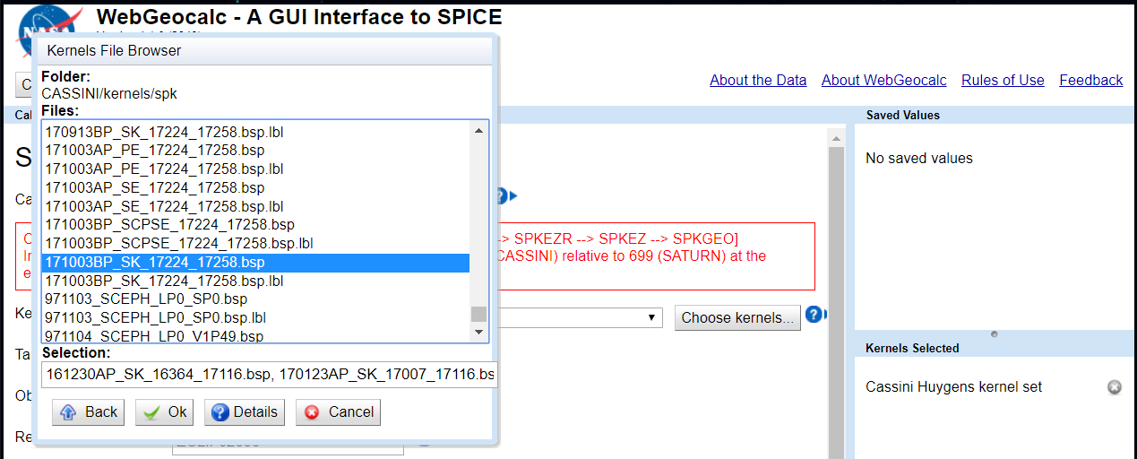
- Go back to the top and under Kernel Selection, click "Manual."
- "Choose Kernels" and navigate to "CASSINI/kernels/spk" and you will be presented with an assortment of confusing filenames of various extensions.
- The readme file can be found here and sheds great insight into the naming
convention that the Cassini team uses for their ephemeris data (something
that often varies by mission). Files produced after May 2003 (which are
what we want) follow the naming convention:
[DeliveryDate][V][T]_[Description]_[StartEvent]_[EndEvent].[Ext]where:[DeliveryDate]is the approximate date that the file was delivered in YYMMDD format[V]is the file version: optional, or may beA,B, etc.[T]is the type of data in the file: optional,Pfor predicted trajectory, orRfor reconstructed trajectory.[Description]is the file description:SKfor orbiter spacecraft trajectory SPK fileOPKfor orbiter and probe trajectory SPK filePEfor planetary ephemeris SPK fileSEfor major satellite ephemeris SPK fileREfor minor satellite ephemeris SPK fileIRREfor outer irregular satellite ephemeris SPK fileSCPSEfor a merged spacecraft, planetary, and satellite ephemerides file
[StartEvent]is the identifier of the file coverage start event, consisting ofYYandDOYwhereYYis the last two digits of the year andDOYis the day of the year. May beNAfor "not applicable".[EndEvent]idenifies the fole coverage end event, in the same format as[StartEvent].[Ext]is the standard SPICE extension for SPK files:bspfor binary SPK files;xsportspfor transfer format SPK files.
We are interested in descriptions that use "SK" for orbiter spacecraft trajectories and start and end events that begin with "17" for the year 2017. The last file should read "17258" for end event indicating September 15, 2017. It is handy to use the delivery date as a means to find the more newly released data sets. The file extension should be ".bsp" not ".bsp.lbl" or other options.
- Select Cassini SK kernels from 2017 as depicted below.
- In the Kernel File Browser, navigate to
pds/wgc/mkand load the latestsolar__system__v****.tmfile (solar__system__v0024.tmat the time of writing).
These should populate the right side of the screen after loaded:
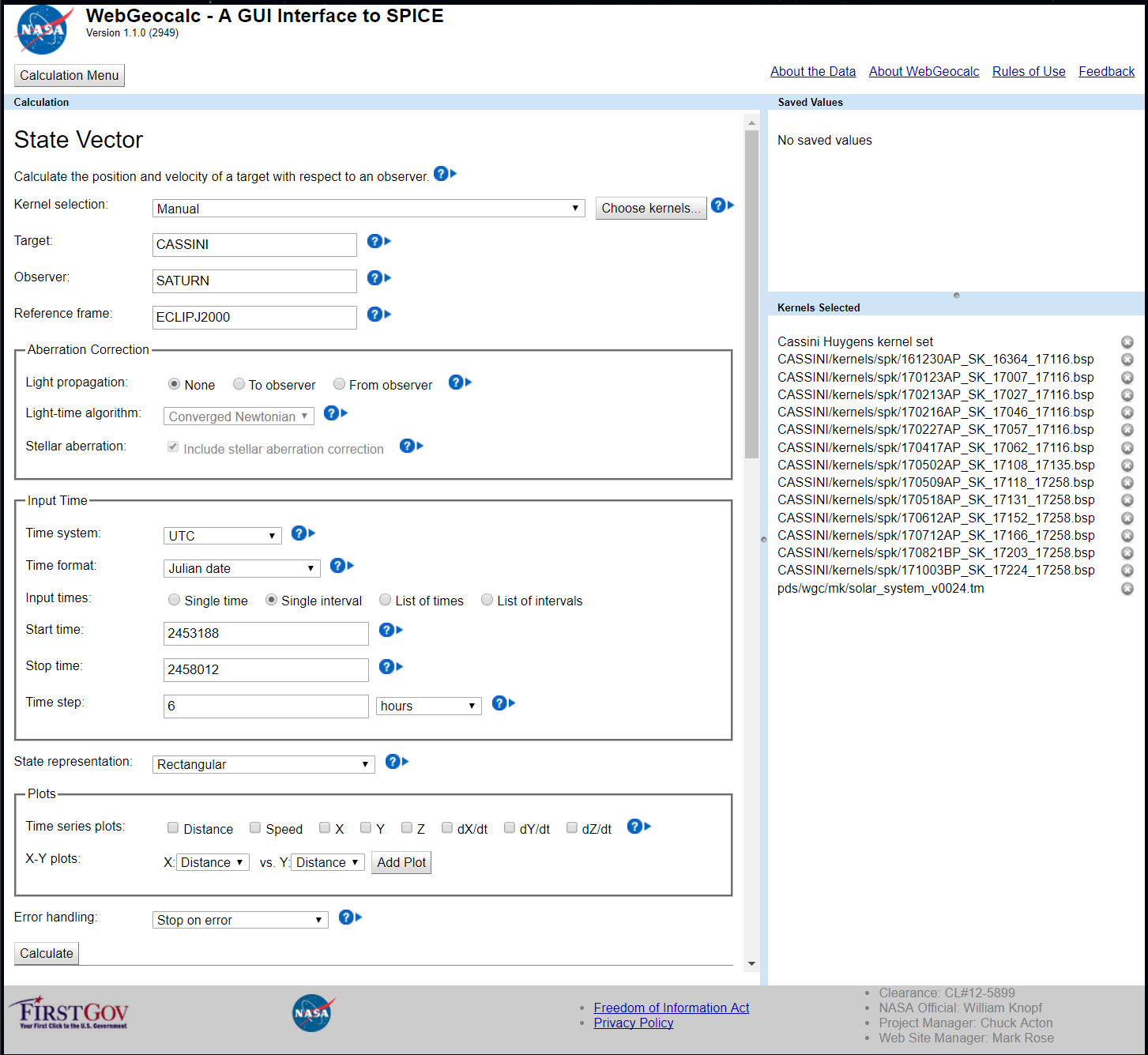
Calculate and troubleshoot errors if necessary. Download the results (I like to use the Excel file version) and then open in Excel. It should look like 19,297 rows of this:
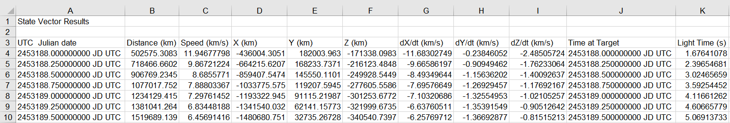
We need columns A, D, E, and F.
- Copy those 4 full columns (without headings/labels) into a second excel
sheet (the first excel sheet is not irrelevant) and using Find and Replace
(CTRL-F): Replace All
JD UTCwith "" (nothing). - Save this new excel sheet as a text file
Cassini.txt - Navigate through the file manager in your computer to this newly created
text file and change the file extension from
.txtto.xyz. Ensure that file extensions are shown in the file manager and that you edit the extension rather than simply the name. This could result inCassini.txtrenamed asCassini.xyz.txt(which will not work, and will not be visible if file extensions are hidden) instead ofCassini.xyz(which will work). - Open AAS WorldWide Telescope and right click on Saturn within the Layer
Manager on the left side of the screen.
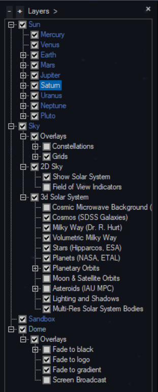
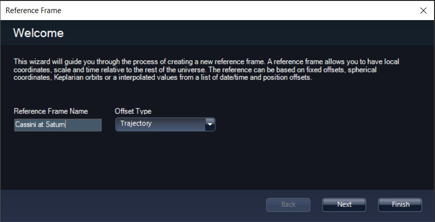
- Click "New Reference Frame" (this can be created for any of these celestial
bodies for future data importation). The following Reference Frame Wizard
will pop up. Name the new reference frame and change the offset type to
"Trajectory."
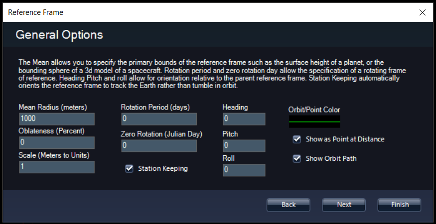
- Clicking "Next" brings you to the following menu. I recommend choosing the
color as lime green as it is easy to see and can be modified later, if
desired. Check the boxes to show the reference frame as a point in the
distance (easy to find) and to show the orbit path (even easier to find).
- The last menu allows you to import the trajectory path that we labored to
create thus far. Simply click import path and navigate to the
Cassini.xyzfile. Be sure to specify "Kilometers" as the units and click finish.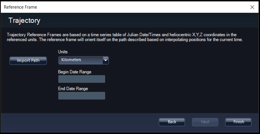
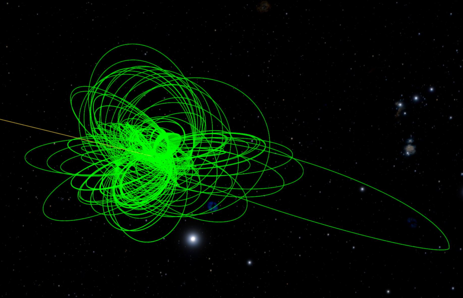
Here is the finished product! Note in the picture below, "Moon & Satellite Orbits" must be checked on in the Layer Manager and then I have turned off each of Saturn's moons by checking them in the Layer Manager (children of the Saturn reference frame). Zooming in, one might find jagged/rough lines that run through the rings of Saturn. This can be fixed by creating a layer with more data points and a smaller time step (1 hour or less). Be sure to save your layers (they will not stay otherwise) by right clicking on the layer in the layer manger and clicking "Save Layers."
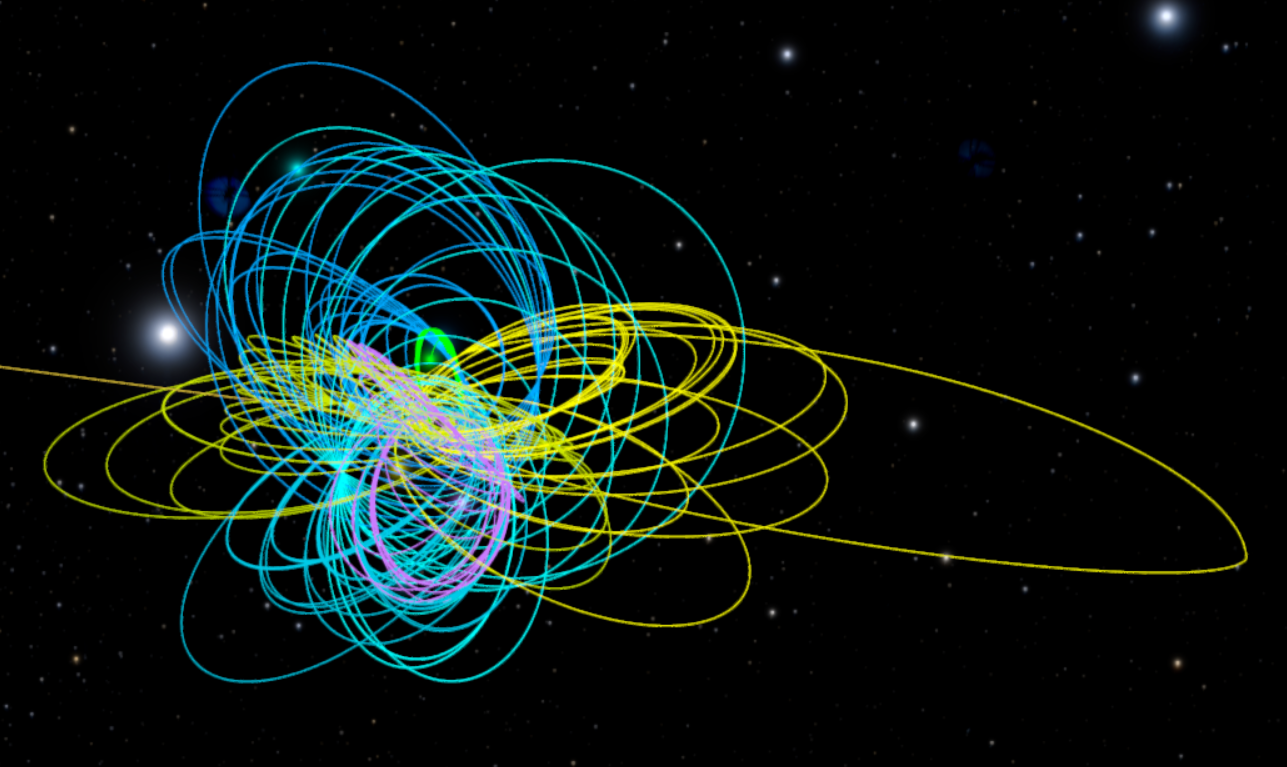
Taking a step further, I've separated the Cassini orbits into color coded sub missions:
Take it another step and modify the input into the WebGeocalc GUI to visualize Cassini's orbit relative to the Sun from launch until orbital insertion or try out any number of different satellites!