Astronomical Image Data Layers

Astronomical images, defined as those with sky coordinate metadata, can be loaded directly into AAS WorldWide Telescope (WWT) in several ways.

Loading Local AVM-tagged Images🔗

Astronomical Visualization Metadata (AVM) is a way to storing information about the original astronomical image in the header of a standard image file, such as TIFF and JPEG. This standard uses existing header infrastructure and populates it with astronomy-specific metadata. The relevant metadata to WWT is:

• Image Name
• URL
• Credits
• Caption
• World Coordinate System (WCS) coordinate information

The idea behind AVM is to allow visualizers to manipulate colors, add annotations etc. and maintain the description of that manipulation – e.g., original data location, color representation – so that subsequent people know how it was created and how to interpret it. For WWT, coordinates allow the image to be placed at the correct location on the sky.

You can download AVM-tagged data from a variety of data sources. If your favorite source of image data provider doesn’t currently include AVM tags, you can direct them to the AVM resources below. If you want to get a test image, you can browse for one on the Astropix website, which aggregates AVM-tagged images. Once you have it, you can add the data to WWT by:

1. Make sure you are in Sky Mode.
2. Under the Explore Tab, click on Open/Astronomical Image…
3. Browse to the appropriate file.
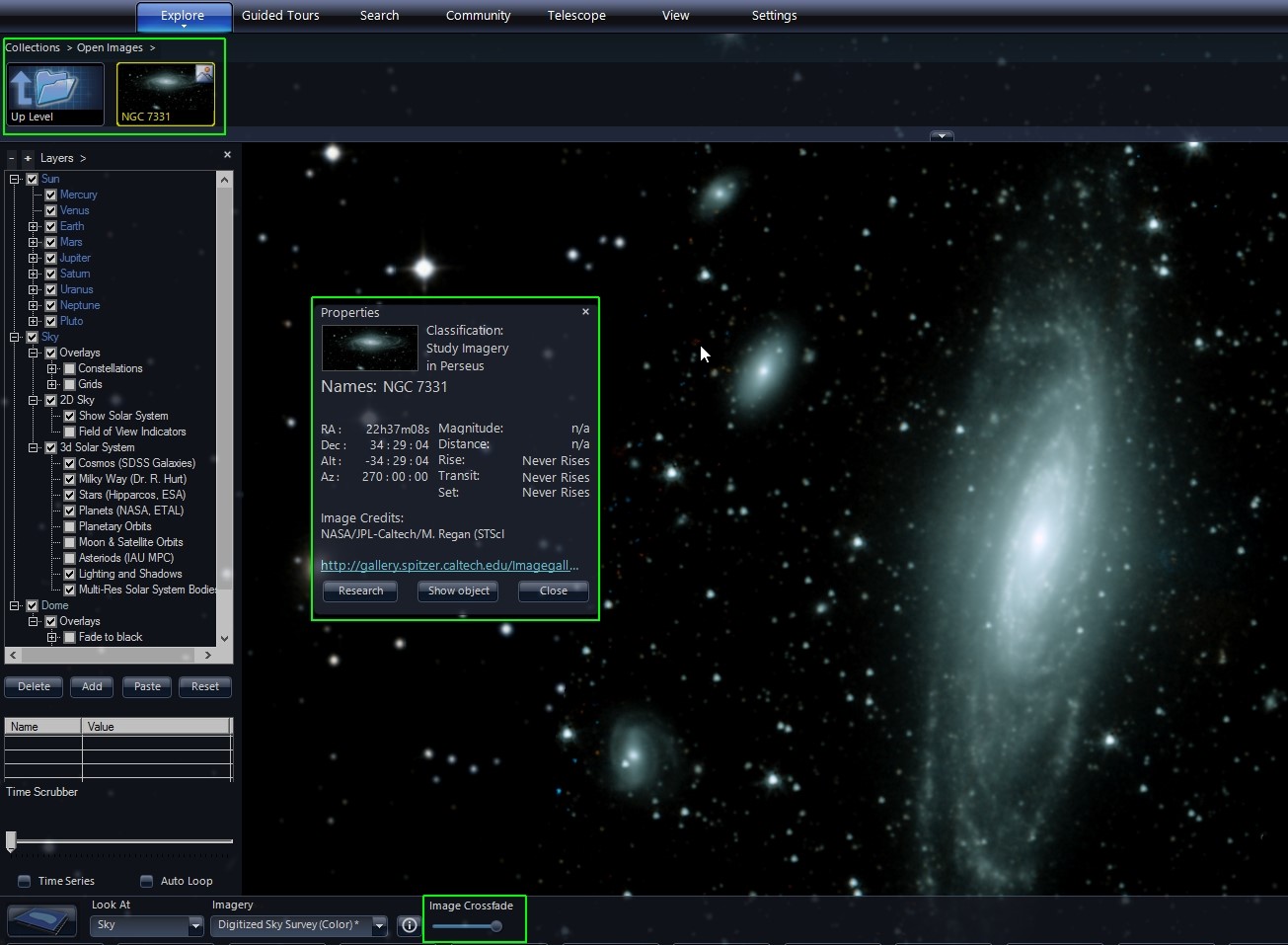
4. WWT will load the data into WWT and add it to a default collection called “Open Collections,” shown in the upper left-hand part of WWT. You can right click and add it to a collection of your choice for image organization after you have loaded it.
5. You can right-click on the image in the collection and select “Properties” to see the image, coordinates, image name, caption, URL. These values are all pulled from the AVM tags when the file is read.
6. You can adjust the cross-fader to change the opacity of this overlaid image on top of the current background.
7. You can also adjust the Image Alignment by pressing CTRL+E to open the Image Alignment instructions.

Loading Remotely-served AVM-tagged Images🔗

In a similar fashion, you can point your browser to an AVM-tagged image on the Internet and it will show the image in your browser in a similar overlay using web controls, with a link to view the image in WWT. Clicking this send this image to the WWT desktop client and allows display control and exploration, similar to interaction with local AVM-tagged Images, above. You can try this out for yourself.

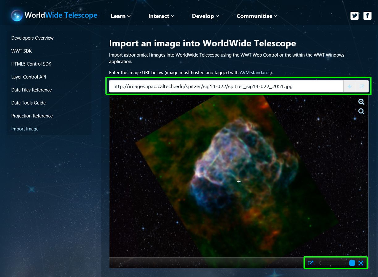
1. Open the following URL in your browser: http://www.worldwidetelescope.org/GetInvolved/ImportImage.
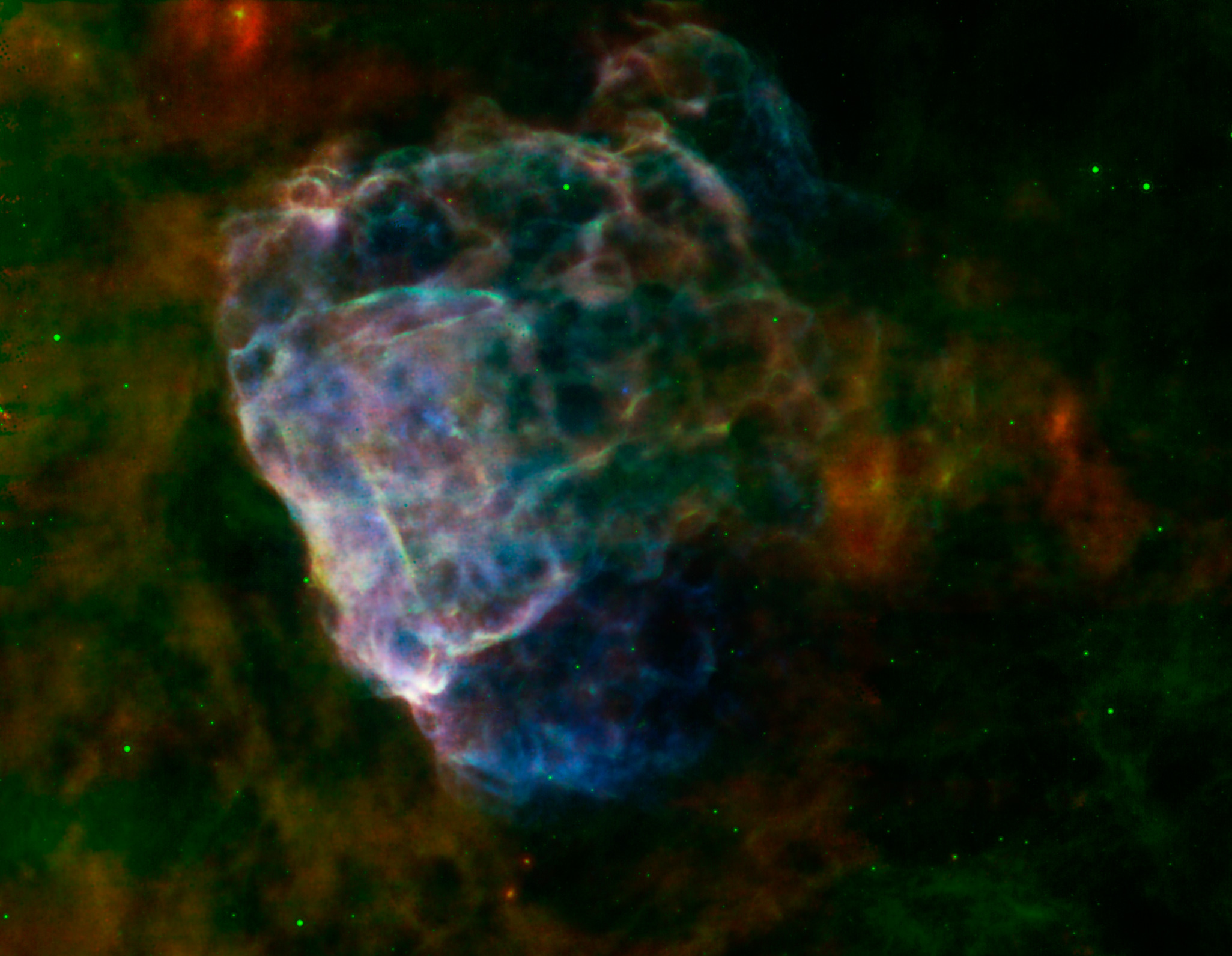
2. Paste the URL to this composite X-ray and Infrared image of Puppis A, which has already been AVM-tagged into the Image URL input field on the webpage: http://images.ipac.caltech.edu/spitzer/sig14-022/spitzer_sig14-022_2051.jpg.
3. This will open the image the webpage with control over image cross-fade and full-screen in the lower right. You can also click the button to the left of the cross-fader which opens the image in the WWT desktop client.

Loading FITS Files🔗

1. Make sure you are in Sky Mode.
2. Under the Explore Tab, click on Open/Astronomical Image…
3. Browse to the appropriate FITS data file. This can be pulled from the Internet or from an attached telescope or a local file.
4. WWT will load the FITS file into WWT and add it to a default collection called “Open Collections,” shown in the upper left-hand part of WWT. You can right click and add it to a collection of your choice for image organization after you have loaded it.
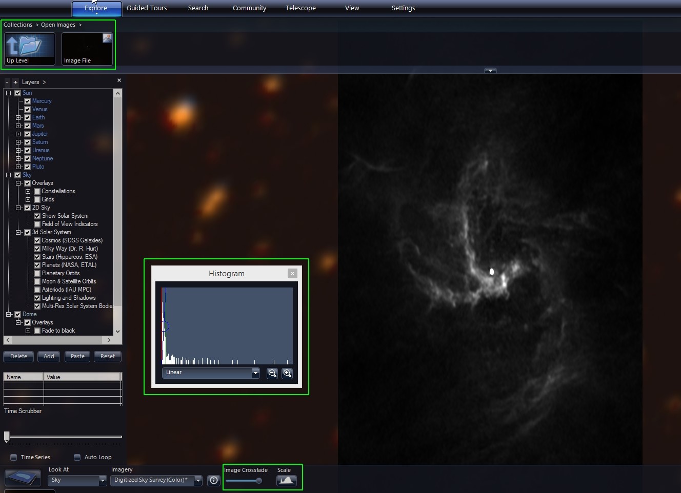
5. Note that FITS files contain pixels, which are mapped to physical coordinates, and data values. To view the image data values must be mapped to colors. The default color map is a linear greyscale one where the lowest value is mapped to black and the highest to white, with linear steps in between. You can interactively adjust this mapping by clicking on the Scale button, which opens the Histogram dialog box.
6. In the Histogram dialog you can select the mapping function between Linear, Log, Power, Square Root and Histogram Equalization.
7. You can change the minimum and maximum data ranges by moving the red and green vertical lines, respectively. If you move the green line to the left of the red line, this inverts the mapping and low values will be show white and high values black.
8. Grabbing the blue circle in the middle will allow you to keep the mapping function width of the function and move it through the histogram left and right.
9. You can adjust the cross-fader to change the opacity of this overlaid image on top of the current background.